In this post, I will show you how to create a drop-down list from a dynamic table located on another sheet within the same workbook. I came across this particular subject when wanting to create a PowerShell script to assign 365 licenses to users from a CSV. The CSV would of course need to contain the userPrincipalname and a list of available licenses in our tenant. That PowerShell script can be found here.

Let’s Begin

This will be a generic list of users and groups.

Create two sheets

Sheet1 will include the user and group columns

Sheet2 will include a list of groups

Sheet2:

• Create the list and select a single cell
• Click Format as Table in the Styles section and choose a style
• Notice all the columns are selected even though you only had one cell selected
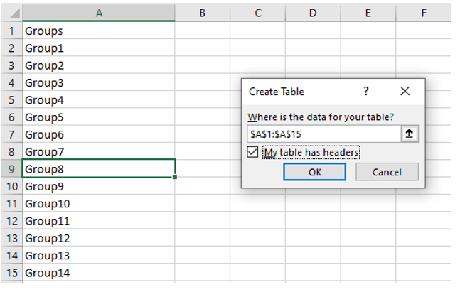
• Check My table has headers and click OK
• This will convert your table to a dynamic table and any additional values that are added to the list will automatically populate in our drop-down

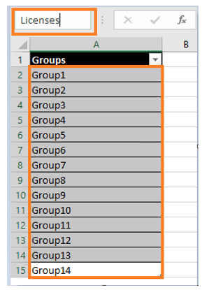
• Select all the columns except for the table header, rename the table and press Enter (*I accidentally typed Licenses instead of Groups – make sure to type the correct name you want to use)

Sheet1:

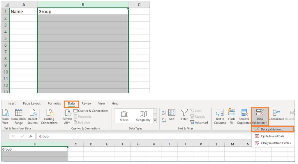
• Highlight the group column
• Select the Data tab, click Data Validation>Data Validation under the Data Tools section

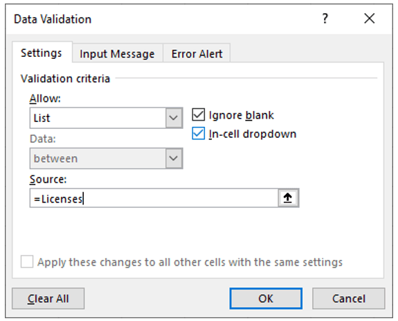
• In the Data Validation dialog box, choose List under the Allow drop-down and type the table name you just created in the Source drop-down as seen below (=TableName)

Verify

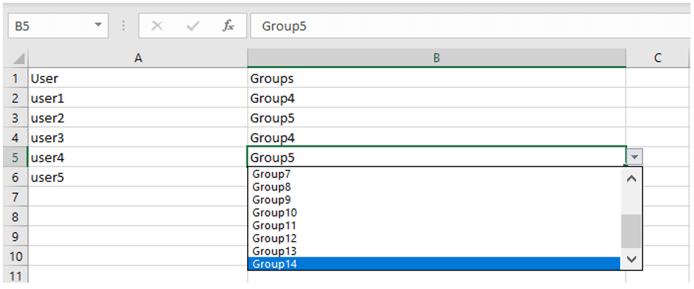
You should now be able to select a choice from the drop-down menu

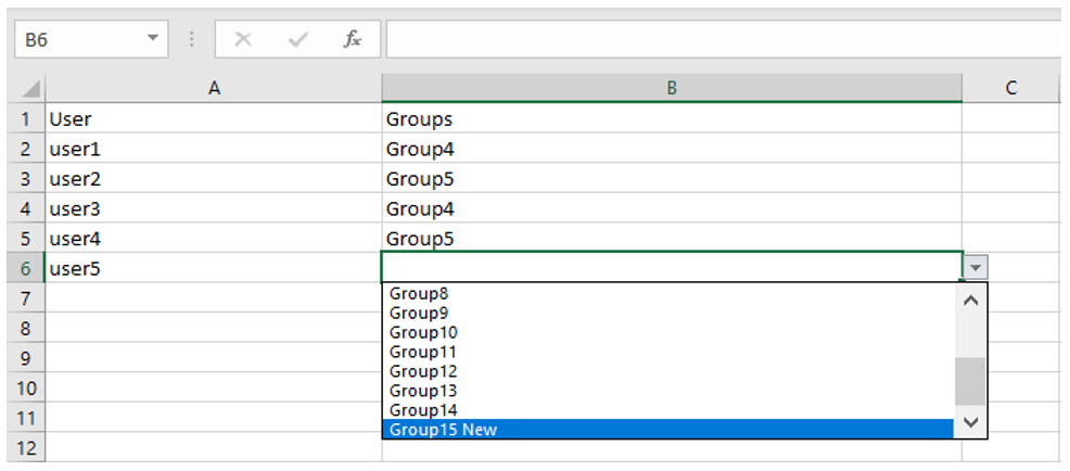
If you go to Sheet2 and add a new group directly beneath the last row, the dynamic table will automatically update on Sheet1

Alternate Method

I’ve tried the method above several times and, 9 times out of 10 it works fine. That 1 time out of 10 is such a mystery to me. I would be presented with the following message when trying to enter the Data Validation:

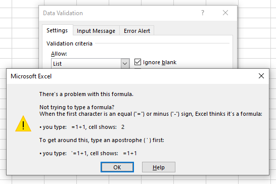
I’ll show you an alternate method that will still accomplish our task.

On our second sheet that contains the list, instead of formatting the table, highlight the list and select Formulas>Define Name. Highlight and copy the Refers to: section, which includes the range you just highlighted. Cancel the New Name dialog box and go to the first sheet.

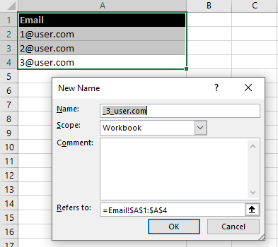
Highlight the column you wish to add the list to and select Data>Data Validation. Select Allow>List and paste the copied data into the Source field. Click OK and now you should see the drop-down list in the column.